Continuous Analysis RNA-Seq Differential Expression Analysis Example using Salmon

This is a sample repository showing a Continuous Analysis Workflow for RNA-Seq analysis. Here, we perform the RNA-seq continuous analysis presented in the Beaulieu-Jones and Greene pre-print using Salmon for RNA-seq quantification.

In this example we follow the workflow described by David Balli and use data generated from Boj et al. (open access). Balli used a similar workflow to the one described by Andrew Mckenzie.

To preform this analysis we use the following tools:

• Salmon
• Limma

Sample Results

The Continuous Analysis process generates several useful artifacts including the following:

1. PCA Plot: 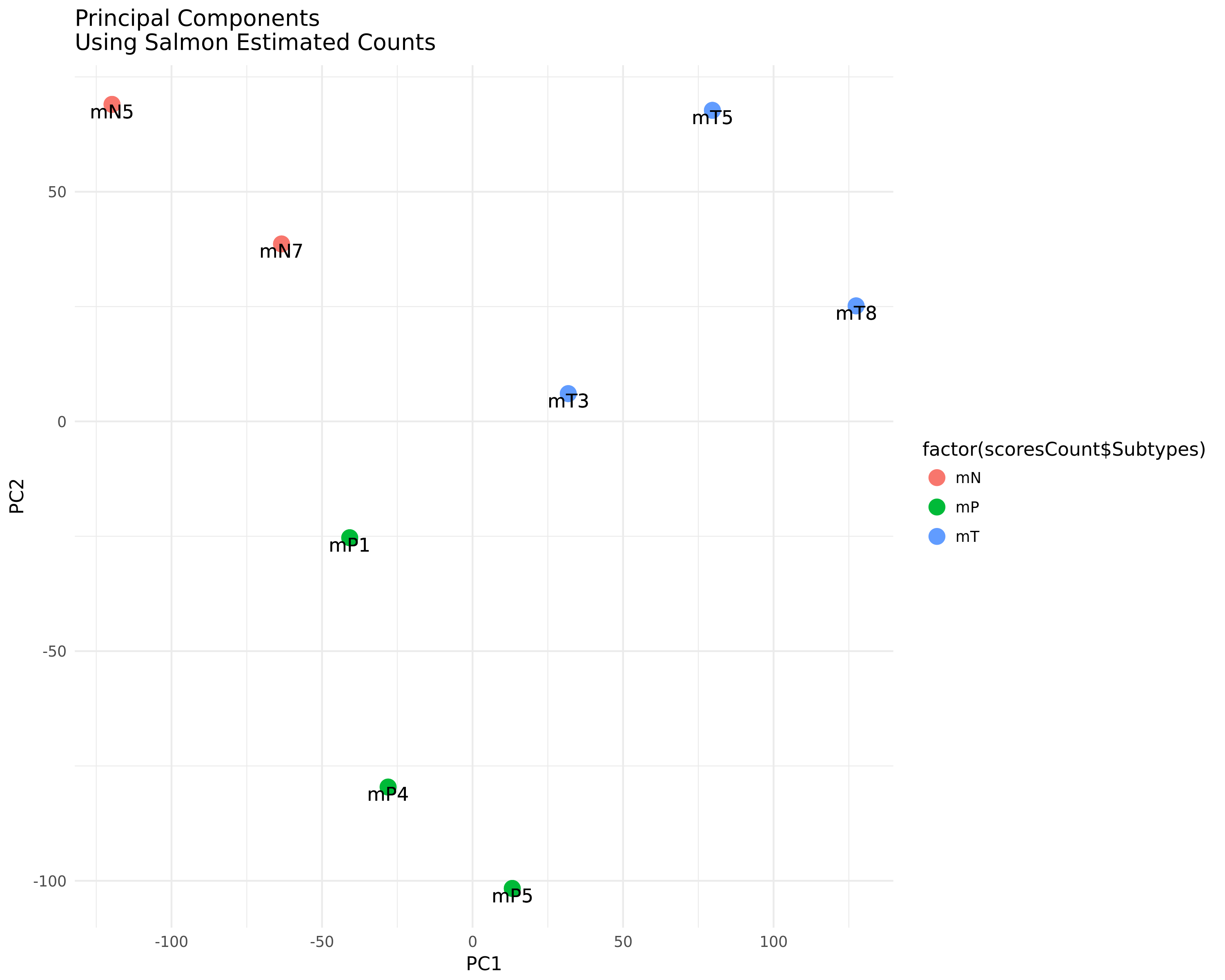A Principle Component Analysis (PCA) of the quantified samples based on Salmon's estimated read count.

2. Volcano Plot of Normal vs. mP samples: 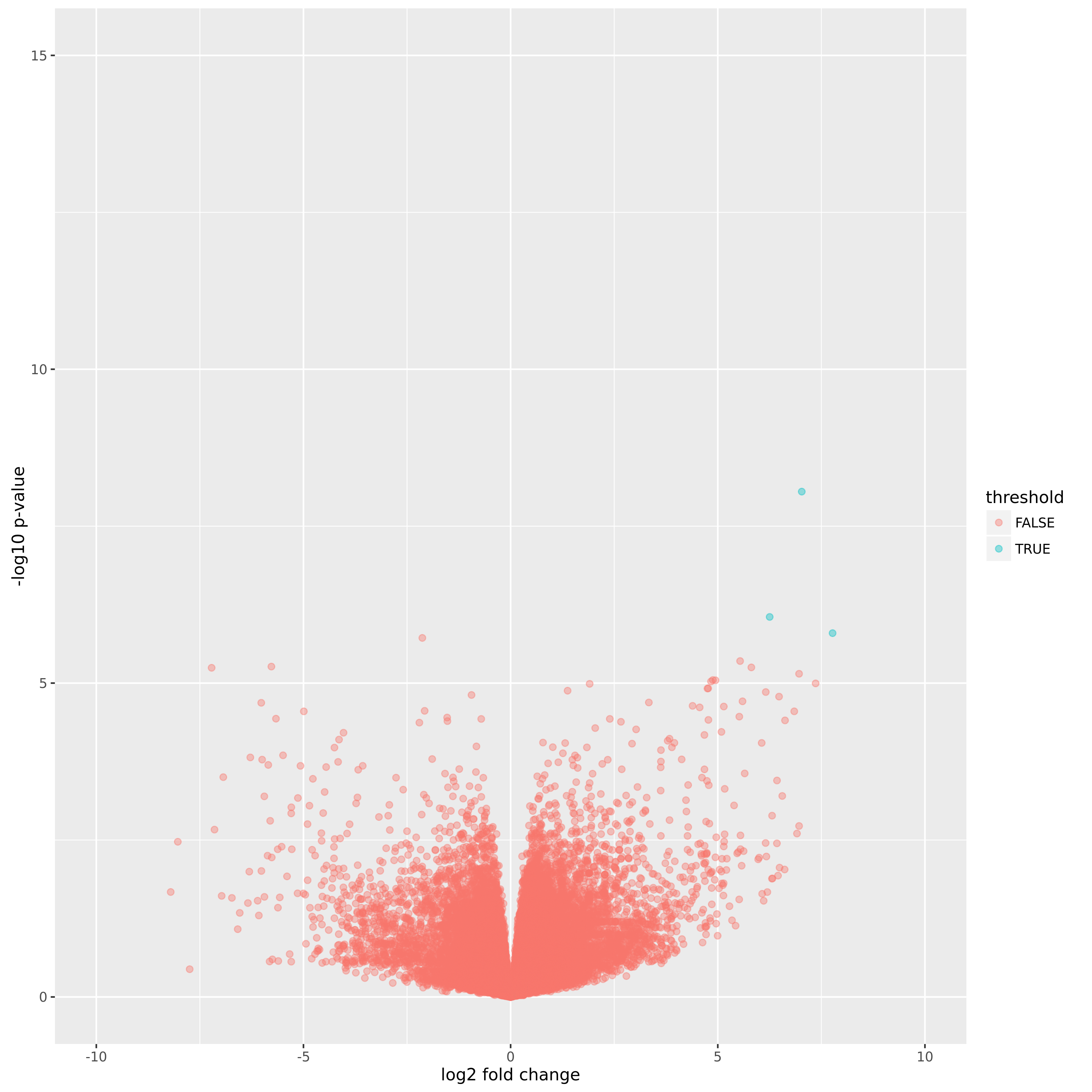A volcano plot plotting the p-value vs. the log fold change.

3. Volcano Plot of Normal vs. mT samples: 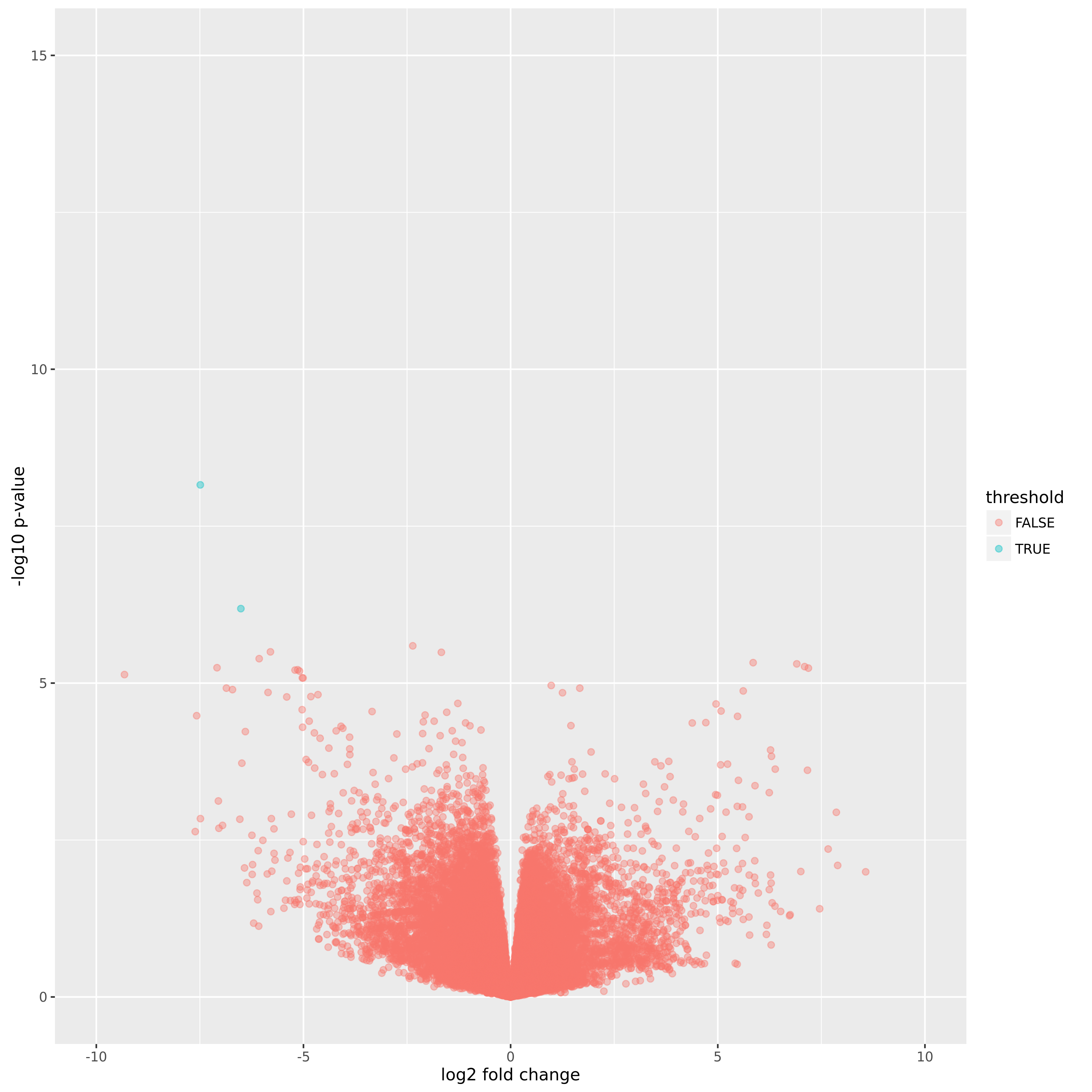A volcano plot plotting the p-value vs. the log fold change.

Description of analysis

We follow the same workflow laid out by Beaulieu-Jones and Greene. A description of this analysis appears below:

We followed a reduced analysis workflow demonstrated by Balli using the SRA files for 8 samples: 2 normal, 3 mP, 3 mT). These samples represent extract to approximately 480 million reads and 150gb of data (FASTQ format). We perform this experiment first with 7 samples (2 normal, 3mP, 2mT) and then add the 8th sample to view the differences.

We perform two preprocessing steps prior to beginning continuous analysis (details/reasoning in continuous analysis configuration section).

Download the samples from the [Sequence Read Archive](http://www.ncbi.nlm.nih.gov/sra?term=SRP049959 "SRR1654626", "SRR1654628", "SRR1654633", "SRR1654636", "SRR16546367", “SRR1654639”, "SRR1654637", "SRR1654641", "SRR1654643") Split the .sra into fast q files using the SRA toolkit Download the mouse reference genome assembly

Continuous Analysis Run (script):

1. Generate a Salmon index file from the reference file and quantify abundances of transcripts from each RNA-Seq sample (run on 28 cores). The Salmon library type was set to -l A to automatically detect the type of each sample.
2. The next portion of the analysis is performed from r_script.r and follows the workflow described by Balli: Generate the transcripts per million (TPM) matrix.
3. Create a matrix to specify the group each sample belongs to.
4. Filter out lowly expressed genes.
5. Generate a principle component plot
6. Fit the limma linear model for differential gene expression analysis.
7. Plot differential expression in the form of a volcano plot.

Feedback

Regarding the original analysis, please email (brettbe) at med.upenn.edu with any feedback or raise a github issue with any comments or questions.

If you have feedback or questions regarding the Salmon pipeline in particular, please e-mail (rob.patro) at cs.stonybrook.edu.

Acknowledgements

We would like to thank David Balli for his post providing the analysis design and significant source code used in this example.

This work is supported by the Gordon and Betty Moore Foundation's Data-Driven Discovery Initiative through Grant GBMF4552 to C.S.G. as well as the Commonwealth Universal Research Enhancement (CURE) Program grant from the Pennsylvania Department of Health.